Parameterizing ARCHI
ParameterizingARCHI.RmdIntroduction
ARCHI provides a flexible platform and modeling workflow or regional-scale imputation of hydrologic records. This article contrasts the different modeling methods provided by ARCHI and highlights some key aspects of model parametrization and evaluation.
How much data is enough?
ARCHI allows users select sites to attempt for imputation based on
the proportion of the record that is complete (not NA)
using the trim_grid() function. For the purposes of this
example, only sites with at least 35 percent of monthly timesteps from
1975 to 2022 will be considered for imputation. This minimum data
threshold requires potential targets to have 16 years worth of monthly
observations within the 47-year period of interest, providing model
training data across a range of hydrologic conditions. There is no
universal rule for how much data is enough for a reliable imputation,
which depends heavily on the correlation structure and missingness
patterns in the dataset. However, ARCHI will not attempt imputation for
sites with less than 10 observation values as regression analysis is
generally considered to be limited on such sparse training data. As a
first-order approximation, it is recommended to begin with a minimum
data threshold of 50 percent and iteratively adjust this value after
inspecting results. ARCHI’s graphical user interface (see
run_gui()) can help practitioners explore the effects of
different data thresholds on model results.
# Gridding groundwater levels by monthly medians from 1975 to 2022
grid <- timestep_grid(data =  LI_data,
                      timestep = "monthly",
                      agg_method = "median",
                      year_range = c(1975, 2022))

# Trim grid to remove sites with less than 35 percent observed values
grid <- trim_grid(input_grid = grid,
                  data_thresh = 0.35)
#> 339 site(s) removed with proportion complete less than site-data threshold of 0.35
Setting an error threshold
ARCHI requires the user specify an error threshold to accept
regression models for imputation. Error methods include: root mean
square error (RMSE), mean absolute error (MAE), normalized root mean
square error (NRMSE), and Nash-Sutcliffe efficiency (NSE). More
information on error methods can be found by entering
?impute_grid in the R console. For RMSE, MAE, and NRMSE,
models will not be accepted if error metrics exceed respective error
thresholds. For NSE, models will not be accepted if they have NSE values
lower than the error threshold. The default for
impute_grid() is an NSE threshold of 0, which requires
models to perform better than mean imputation. Increasing the NSE
threshold raises the bar for model acceptance, with 1 indicating a
perfect model fit (observed values equivalent to modeled values).
To explore the effects of the error threshold on model results, the user can test a range of error thresholds ranging from loose (NSE = 0) to more stringent (NSE = 0.8).
# Create empty list for model outputs
mods_out <- NULL

# Run models with NSE error thresholds of 0, 0.2, 0.4, 0.6, and 0.8
threshs <- c(0,0.2,0.4,0.6,0.8)

for(i in seq(1,length(threshs))){
mods_out[[i]] <- impute_grid(input_grid = grid,
                             model = "OLS",
                             n_refwl = 10,
                             error_method = "NSE",
                             error_thresh = threshs[i])
}

# Save all model fits to a data frame
fits <- data.frame("NSE0" = mods_out[[1]]$model_stats$NSE,
                   "NSE0.2" = mods_out[[2]]$model_stats$NSE,
                   "NSE0.4" = mods_out[[3]]$model_stats$NSE,
                   "NSE0.6" = mods_out[[4]]$model_stats$NSE,
                   "NSE0.8" = mods_out[[5]]$model_stats$NSE
                   )
# Any accepted model will have an error metric associated with it
# Sites that were not successfully imputed will have NA under the NSE field

# Plot mean model fits by error threshold
plot(threshs, apply(fits,2,mean,na.rm=T), type = 'b',
     xlab = "Model error threshold (NSE)", ylab = "Mean fitted NSE",
     cex = 1.4, lwd = 2, cex.lab = 1.4, cex.axis = 1.2)
Tightening the error threshold excludes models with poorer fits, increasing the mean fitted NSE value.
However, too stringent a threshold can result in very few to no sites being successfully imputed. Only two sites were imputed when the NSE threshold was set to 0.8.
# Plot number of successful imputation models by error threshold
plot(threshs, 100 * colSums(!is.na(fits))/dim(fits)[1],type='b',
     xlab="Model error threshold (NSE)",
     ylab = "Percent of target sites successfully imputed",
     cex = 1.4, lwd = 2, cex.lab = 1.4, cex.axis = 1.2)
Ultimately, it is up to the user to evaluate which error thresholds
best satisfy their modeling goals. Too loose error thresholds could
result in artifacts of poor model fits being propagated through the
dataset. Too stringent thresholds can result in fewer imputed sites,
which may cause information loss whereby fewer references are available
to train subsequent models. As a first-order approximation, it is
recommended to tighten the error threshold until a dropoff in the
proportion of imputed sites is observed (NSE = 0.4, above). ARCHI’s
graphical user interface (see run_gui()) can help
practitioners explore the effects of different error thresholds on model
results.
Comparing regression models
ARCHI utilizes three types of regression model: ordinary least
squares (OLS), ridge regression (ridge), and maintenance of variance,
type 1 (MOVE.1). OLS is a parametric regression method and can be prone
to over-fitting (variance inflation) when too many predictors (reference
sites) are used. Such models can have very good fits to the training
data, but perform poorly on holdout data. Ridge regression overcomes
this issue by application a penalty parameter that decreases the model
variance in exchange for an increase in bias (Hastie, 2020).
ARCHI uses the R package glmnet
to automatically fit the penalty parameter by cross-validation. The
MOVE.1 model maintains the variance of the target record, but can only
use one reference site to train regression models. Alternately, OLS and
ridge can use multiple references to train regression models. In this
section, we will compare these three models using holdout data and
highlight some additional functionality of ARCHI.
# Set seed for reproducibility of holdout dataset
set.seed(123)

# Randomly sample 5 percent of training data
hold <- hold_grid(grid, p = 0.05)

# First we will fit OLS and ridge regression models. Because they are multiple
# regression models, we must specify the maximum number of reference sites that
# can be used to build the model (n_refwl). We will set to "max" to use all
# available correlated reference sites to fit models.
# The default error threshold (NSE = 0) is used below..
OLS_max <- impute_grid(input_grid = hold,
                       model = "OLS",
                       n_refwl = "max")

ridge_max <- impute_grid(input_grid = hold,
                         model = "ridge",
                         n_refwl = "max")

# Because OLS is prone to overfitting, we can use an additional parameter,
# "p_per_n" to limit the number of references used based on the number
# of observed values. Setting p_per_n to 0.10 limits the number of predictors
# (reference sites) to a maximum of one for every 10 observations used to train the model.
OLS_limited <- impute_grid(input_grid = hold,
                         model = "OLS",
                         n_refwl = "max",
                         p_per_n = 0.10)

# We will also use the MOVE.1 model. It is not necessary to specify
# n_refwl because it only allows 1 one reference site per model
MOVE.1 <- impute_grid(input_grid = hold,
                         model = "MOVE.1")
Let’s compare the results of these four different models. We will look at both the overall model fits (RMSE) and their variance ratios (ratio of modeled to observed record variance).
# Save all model fits to a data frame
fits <- data.frame("OLS_max" = OLS_max$model_stats$NSE,
                   "OLS_limited" = OLS_limited$model_stats$NSE,
                   "ridge_max" = ridge_max$model_stats$NSE,
                   "MOVE.1" = MOVE.1$model_stats$NSE
                   )

# Boxplot of accepted model fits
boxplot(fits,
        xlab = "Model type", ylab = "Nash-Sutcliffe efficiency (NSE)",
        cex.lab = 1.4, cex.axis = 1.2)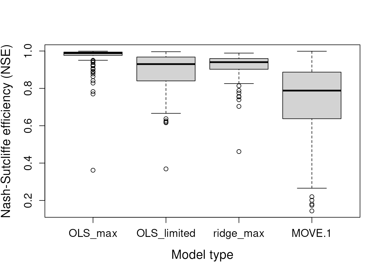
# Save variance ratios to a data frame
vars <- data.frame("OLS_max" = OLS_max$model_stats$var_ratio,
                   "OLS_limited" = OLS_limited$model_stats$var_ratio,
                   "ridge_max" = ridge_max$model_stats$var_ratio,
                   "MOVE.1" = MOVE.1$model_stats$var_ratio
                   )
# Boxplot of variance ratios
boxplot(vars,
        xlab = "Model type", ylab = "Variance ratio (modeled/observed)",
        cex.lab = 1.4, cex.axis = 1.2)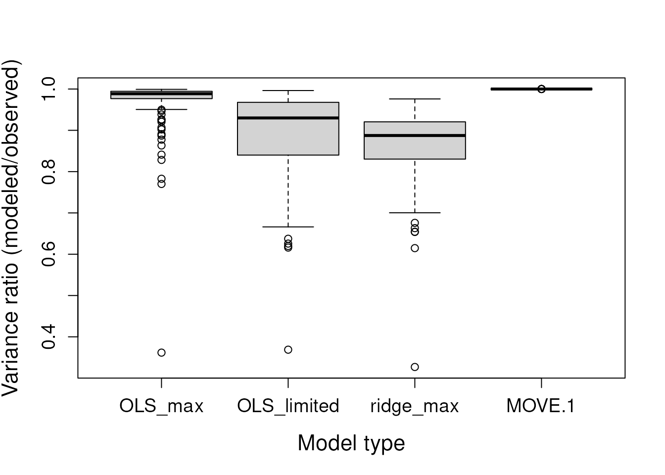
The “OLS_max” model shows the best apparent fits to the training data, as measured by the NSE. The “MOVE.1” model, as expected, preserves the variance of the training data (variance ratio = 1). The “ridge_max” model results in the greatest variance loss due to the application of the penalty parameter. Now, let’s examine the holdout data.
# Evaluate holdout data
eval1 <- hold_eval(true = grid, imp = OLS_max$imputed_grid, hold = hold)
eval2 <- hold_eval(true = grid, imp = OLS_limited$imputed_grid, hold = hold)
eval3 <- hold_eval(true = grid, imp = ridge_max$imputed_grid, hold = hold)
eval4 <- hold_eval(true = grid, imp = MOVE.1$imputed_grid, hold = hold)

# Create data frame of difference vectors
diffs <- data.frame("OLS_max" = eval1$diff,
                    "OLS_limited" = eval2$diff,
                    "ridge_max" = eval3$diff,
                    "MOVE.1" = eval4$diff
                   )

# Only include complete cases where holdouts were imputed by all models
# Note: all candidate sites were imputed by all models except MOVE.1, which
# did not impute 3 of the 137 sites with missing data
diffs <- na.omit(diffs)

# Compute RMSEs for holdouts imputed across all model runs
rmses <- apply(diffs, 2, function(x) sqrt(mean(x^2)))

rmses
#>     OLS_max OLS_limited   ridge_max      MOVE.1
#>   1.2073852   1.0887156   0.9629651   1.8456351

# Plot model comparison holdout data fits
plot(c(1:length(rmses)), rmses, type='b',
     xlab="Model type",
     ylab = "Holdout RMSE, in feet",
     cex = 1.4, lwd = 2, cex.lab = 1.4, cex.axis = 1.2, xaxt = "n")
axis(1, at = c(1:length(rmses)), labels = names(rmses), cex.axis= 1.2)
Although the “OLS_max” model had the best apparent fits to the training
data, the “ridge_max” model was the most generalizable to the holdout
data. Although “MOVE.1” had the poorest apparent fits and holdout
errors, it effectively preserves the variance of the target record,
which can be useful for specific statistical applications.
References
Hastie, T., 2020, Ridge Regularization: An Essential Concept in Data Science: Technometrics, v. 62, no. 4, p. 426-433, https://doi.org/10.1080/00401706.2020.1791959.