Troubleshooting ARCHI • ARCHI

Introduction

ARCHI provides a flexible platform and modeling workflow for regional-scale imputation of hydrologic records. This article highlights some challenges users might face implementing ARCHI and suggests some simple fixes. The following example examines a case where ARCHI fails to impute a dataset.

library(ARCHI)

# Load ARCHI example data
data(LI_data) # Groundwater-level values, in feet below land surface
data(LI_sites) # Site metadata with coordinates referenced to NAD83

# Gridding groundwater levels by monthly medians from 1975 to 2022
grid <- timestep_grid(data =  LI_data,
                      timestep = "monthly",
                      agg_method = "median",
                      year_range = c(1975, 2022))

# Trim grid to remove sites with less than 35 percent observed values
grid <- trim_grid(input_grid = grid,
                  data_thresh = 0.35)
#> 339 site(s) removed with proportion complete less than site-data threshold of 0.35

# Set add_std_means to FALSE (default is TRUE)
mod_fail <- impute_grid(input_grid = grid,
                       model = "ridge",
                       error_method = "NSE",
                       error_thresh = 0,
                       n_refwl = 10,
                       sites = LI_sites,
                       add_std_means = FALSE)
#> Begin initial imputation: 39.46 percent NAs remaining...
#> Iteration 1 complete: 39.46 percent NAs remaining
#> Begin final pass: overwriting initial imputations with improved models...
#> Iteration 2 complete: 39.46 percent NAs remaining
#> Records attempted for imputation =  137
#> Incomplete records remaining =  137
#> Time difference of 0.8847606 secs

Why won’t it work?

There are a few primary reasons why ARCHI may not be able to impute a given dataset. The first is that insufficient correlations exist among the considered records to develop regression models. Another is that the error threshold is too stringent to accept model results. Finally, a common issue is data coverage. ARCHI works best when there are a large proportion of complete or near-complete records present in the initial dataset to help seed the model.

Let’s explore why the above model may have failed. The mod_notes field of the model_stats data frame included in the impute_grid output can help us better understand what happened.

# Create a table showing counts of unique model notes
table(mod_fail$model_stats$mod_notes)
#> 
#> Insufficient data in reference records to fill gaps in target record 
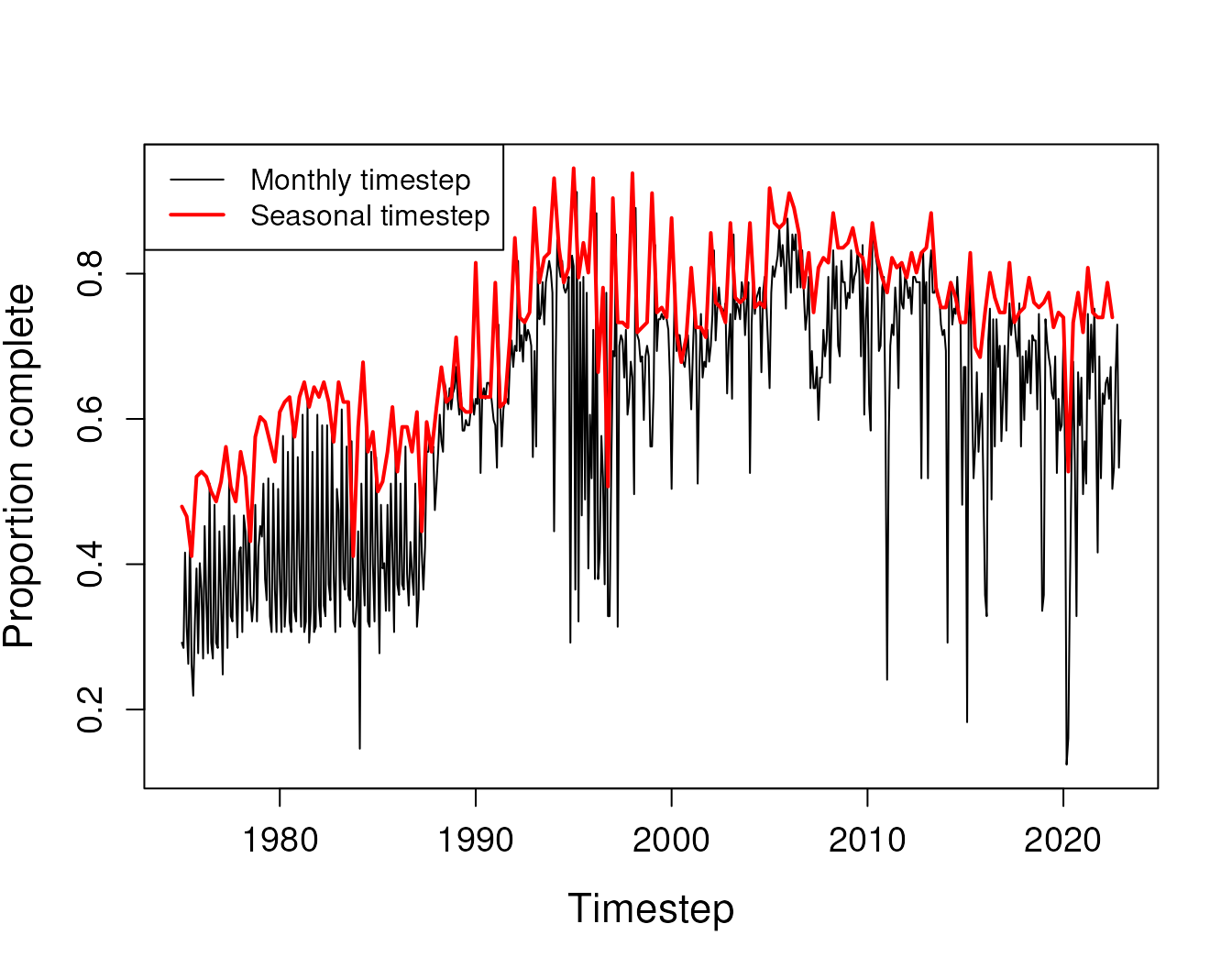
#>                                                                  137

All 137 sites included in the input grid had insufficient data for gap filling. This is most likely due to periods of the input with very sparse data. Because ARCHI requires references have data to fill all gaps in target records, a handful of data-sparse timesteps may bottleneck expansion of the reference pool. We can see some timesteps have very low proportions of sites with data, particularly March 2020.

# Count number of observations in every row (timestep), excluding the leading timestep index column
prop_tstep <- rowSums(!is.na(grid)[,-1])/(dim(grid)[2]-1)

# The timestep with the least amount of data is March 2020 
# Only 12 percent of sites had observed values in that month
prop_tstep[which.min(prop_tstep)]
#>       543 
#> 0.1240876
grid$timestep[which.min(prop_tstep)]
#> [1] "2020-03-01"

# Plot the proportion of sites with data for each timestep
plot(grid$timestep, prop_tstep, type = 'l',
     xlab = "Timestep", ylab =  "Proportion complete",
     cex.lab = 1.4, cex.axis = 1.2)
# Add a point at March 2020
points(grid$timestep[which.min(prop_tstep)],
       prop_tstep[which.min(prop_tstep)], 
       cex = 1.5, col = "red", lwd = 2)

# We can also explore data density using the grid_heatmap() function
# plotly::ggplotly creates interactive html widget that allows user to zoom in
# Add a dashed line at March 2020
hm <- grid_heatmap(grid, cb_rng = c(-3,3))
plotly::ggplotly(hm$grid_plot + 
                 ggplot2::geom_vline(xintercept = which.min(prop_tstep),
                                     linetype =3)
         )

Possible Solutions

In the following sections, we will explore three potential solutions to the data sparsity issue.

1. Add group means

ARCHI can create synthetic references to seed initial imputation models if the add_std_means input to impute_grid() is set to TRUE. This is accomplished by averaging standardized (z-scored by site) observation values across the dataset or by user-specified groups. By default a complete reference record named all_sites is generated, which represents the mean deviation of site records from average conditions during the period of interest. If a grouping variable is supplied in the site metadata, each unique group is also used to generate additional synthetic references, which are attributed with the user-specified group label. Site groupings selected by the user may be used to define reference records representative of different geospatial boundaries or aquifer depth zones.


# Set add_std_means to default of TRUE
mod_out <- impute_grid(input_grid = grid,
                       model = "ridge",
                       error_method = "NSE",
                       error_thresh = 0,
                       n_refwl = 10,
                       sites = LI_sites,
                       add_std_means = TRUE)
#> Begin initial imputation: 39.46 percent NAs remaining...
#> Iteration 1 complete: 0 percent NAs remaining
#> Iteration 2 complete: 0 percent NAs remaining
#> Begin final pass: overwriting initial imputations with improved models...
#> Iteration 3 complete: 0 percent NAs remaining
#> Records attempted for imputation =  137
#> Incomplete records remaining =  0
#> Time difference of 27.32737 secs

Success! Let’s explore the model output

# Explore model output to find data frame of synthetic references
str(mod_out$std_means)
#> 'data.frame':    576 obs. of  4 variables:
#>  $ timestep   : Date, format: "1975-01-01" "1975-02-01" ...
#>  $ Long_Island: num  0.4531 0.2162 -0.028 -0.0469 -0.1009 ...
#>  $ Mainland   : num  -1.125 -0.952 -1.131 -0.714 -0.492 ...
#>  $ all_sites  : num  0.019 -0.113 -0.241 -0.217 -0.22 ...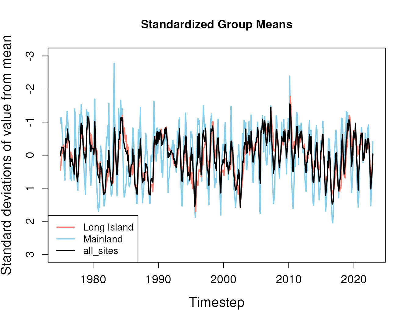

Correlations with these standardized group means can help “seed” the initial imputation model if few complete records exist.

2. Truncate period

The modeling period may be adjusted to exclude data-sparse timesteps. Here, we adjust year_range in the timestep grid function to exclude 2020.

# Gridding groundwater levels by monthly medians from 1975 to 2019, excluding March 2020
grid_trunc <- timestep_grid(data =  LI_data,
                           timestep = "monthly",
                           agg_method = "median",
                           year_range = c(1975, 2019))

# Trim grid to remove sites with less than 35 percent observed values
grid_trunc <- trim_grid(input_grid = grid_trunc,
                        data_thresh = 0.35)
#> 341 site(s) removed with proportion complete less than site-data threshold of 0.35

# Impute truncated grid
mod_trunc <- impute_grid(input_grid = grid_trunc,
                         model = "ridge",
                         error_method = "NSE",
                         error_thresh = 0,
                         n_refwl = 10,
                         add_std_means = F)
#> Begin initial imputation: 38.84 percent NAs remaining...
#> Iteration 1 complete: 0.3 percent NAs remaining
#> Iteration 2 complete: 0 percent NAs remaining
#> Iteration 3 complete: 0 percent NAs remaining
#> Begin final pass: overwriting initial imputations with improved models...
#> Iteration 4 complete: 0 percent NAs remaining
#> Records attempted for imputation =  135
#> Incomplete records remaining =  0
#> Time difference of 21.72118 secs

Success! We could also use trim_grid() to remove data sparse timesteps by adjusting the time_thresh input, but this can create datasets of irregular frequency that may not accurately reflect time-series dynamics within a period of interest.

3. Grid coarser timesteps

We can change our timestep frequency from monthly to seasonal (every three months) to improve data coverage.

# Grid groundwater levels at a seasonal timestep from 1975 to 2022
# This aggregates data into a four-season water year beginning in October 
grid_seas <- timestep_grid(data =  LI_data,
                           timestep = "seasonal",
                           agg_method = "median",
                           type_year = "water",
                           start_month = 10,
                           n_seasons = 4,
                           year_range = c(1975, 2022))
grid_seas$timestep[1:5]
#> [1] "1975-01-01" "1975-04-01" "1975-07-01" "1975-10-01" "1976-01-01"

# Trim grid to remove sites with less than 45 percent observed values
# Approximately same number of sites with sufficient data compared to monthly grid
grid_seas <- trim_grid(input_grid = grid_seas,
                        data_thresh = 0.45)
#> 330 site(s) removed with proportion complete less than site-data threshold of 0.45

We can see that using a seasonal grid for the data has improved temporal coverage substantially.

Now, let’s impute the seasonal grid.

# Impute seasonal grid
mod_seas <- impute_grid(input_grid = grid_seas,
                         model = "ridge",
                         error_method = "NSE",
                         error_thresh = 0,
                         n_refwl = 10,
                         add_std_means = F)
#> Begin initial imputation: 28.3 percent NAs remaining...
#> Iteration 1 complete: 0 percent NAs remaining
#> Iteration 2 complete: 0 percent NAs remaining
#> Begin final pass: overwriting initial imputations with improved models...
#> Iteration 3 complete: 0 percent NAs remaining
#> Records attempted for imputation =  138
#> Incomplete records remaining =  0
#> Time difference of 27.62071 secs

Success!

Conclusions

Different datasets with varied missingness patterns and correlation structures will need to be handled differently. ARCHI provides a flexible and transparent interface for assessing modeling issues, iterative pre- and post-processing, and viewing results.