
![]()
![]()
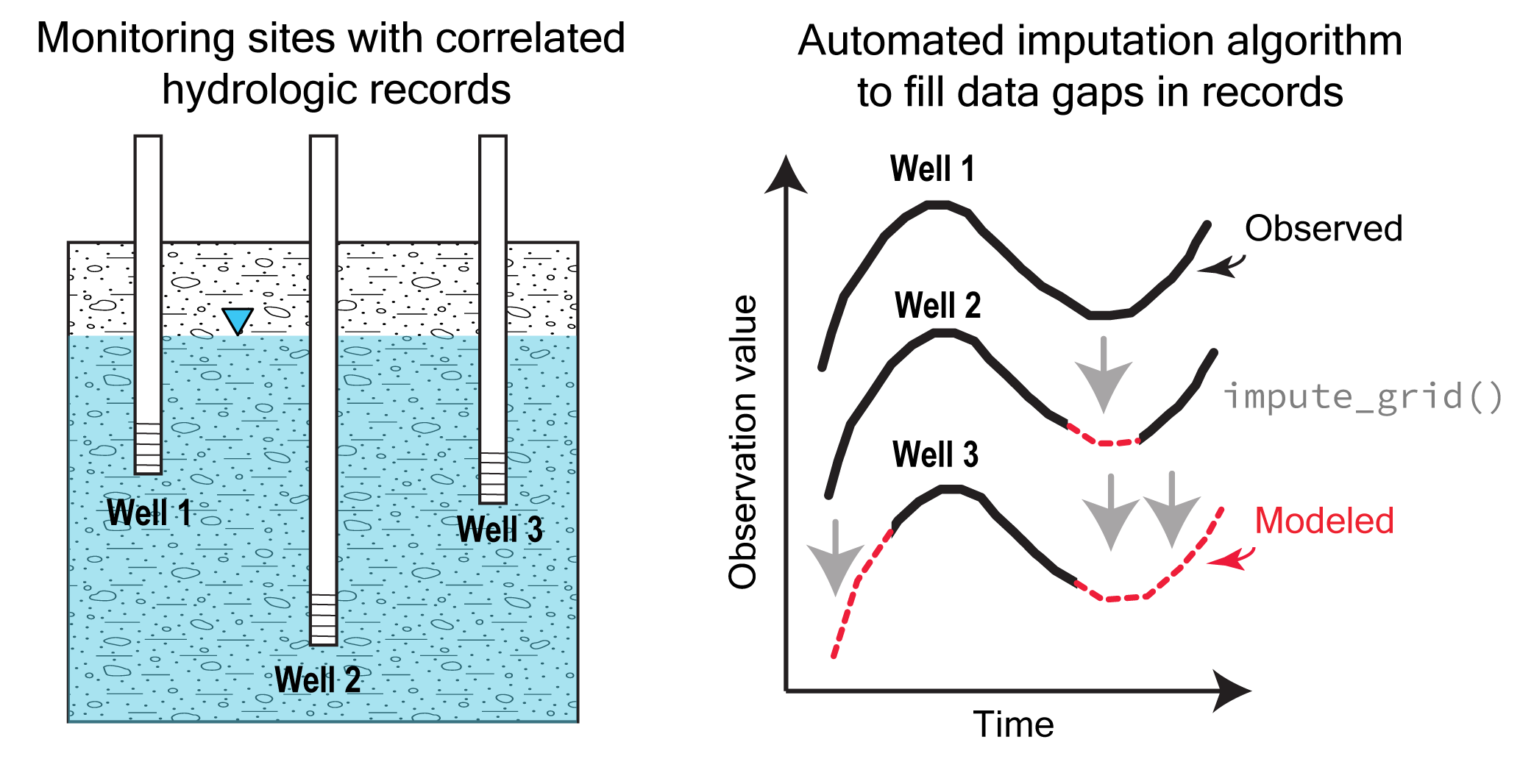
Welcome to Automated Regional Correlation Analysis for Hydrologic Record Imputation (ARCHI). ARCHI provides a workflow and interactive platform for regional-scale hydrologic record imputation. ARCHI allows users to aggregate, visualize, and impute records with irregular monitoring frequency at annual, seasonal, monthly, weekly, and daily timesteps. Missing data at “target” sites are imputed using regression models using more complete “reference” sites as predictors. ARCHI employs an iterative algorithm that allows each site to be considered as either a target or a reference, growing the pool of potential reference sites with each imputation until gap-filling ceases. A user-specified error threshold is used to determine whether regression model results will be accepted and propagated into the dataset. Reference selection can be constrained with distance, correlation, and group-based filters. ARCHI provides additional functions for visualizing results and evaluating model performance with holdout data.
See https://water.code-pages.usgs.gov/ARCHI/ for more information!
Suggested Software Citation
Levy, Z.F., Stagnitta, T.J., and Glas, R.L., 2024, ARCHI: Automated Regional Correlation Analysis for Hydrologic Record Imputation, v1.0.0: U.S. Geological Survey software release, https://doi.org/10.5066/P1VVHWKE.
Suggested Method Citation
Levy, Z.F., Glas, R.L., Stagnitta, T.J., and Terry, N., 2025, ARCHI: A New R Package for Automated Imputation of Regionally Correlated Hydrologic Records: Groundwater, https://doi.org/10.1111/gwat.13474.
Contributors
- Zeno F. Levy (zlevy@usgs.gov): U.S. Geological Survey, California Water Science Center
- Timothy J. Stagnitta (tstagnitta@usgs.gov): U.S. Geological Survey, New York Water Science Center
- Robin L. Glas (rglas@usgs.gov): U.S. Geological Survey, New York Water Science Center
Installing ARCHI
You can install the ARCHI package using the remotes package.
To install the remotes package, copy the following line into R or the “Console” window in RStudio:
install.packages("remotes")To install the ARCHI package:
remotes::install_gitlab("water/ARCHI",
                        host = "code.usgs.gov",
                        build_opts = c("--no-resave-data",
                                       "--no-manual"),
                        build_vignettes = TRUE,
                        dependencies = TRUE)
This will install ARCHI and associated dependencies. You may be prompted to update dependencies, but this is not required.
Getting started with ARCHI: Example workflow
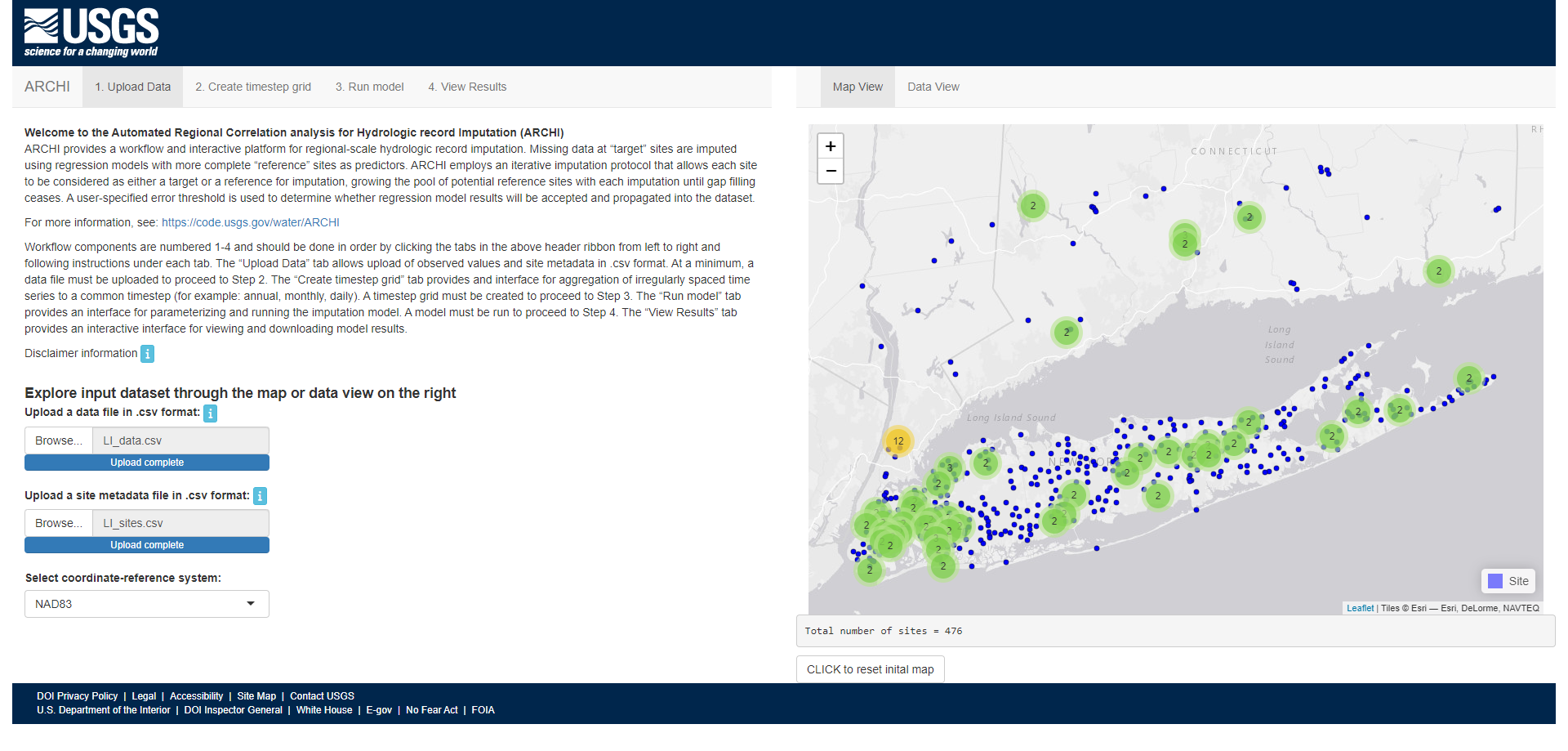
ARCHI is packaged with an example dataset of groundwater-level observations from sites on Long Island, NY and additional coastal “mainland” sites in New York and Connecticut. Groundwater-level values are indexed by site with observation dates ranging from 1975 to 2022. Site metadata includes location coordinates in decimal degrees and an additional nominal group field.
Load example dataset:
library(ARCHI)

# Load example groundwater-level data data frame
# Note the date column is formatted as an R "Date" class
data(LI_data)
str(LI_data)
#> 'data.frame':    89997 obs. of  3 variables:
#>  $ site_no: chr  "403442073575401" "403442073575401" "403442073575401" "403442073575401" ...
#>  $ date   : Date, format: "1980-06-24" "1980-09-23" ...
#>  $ value  : num  7.95 8.11 9.23 8.23 8.02 7.76 7.77 7.81 7.9 7.63 ...

# Load example site metadata data frame
data(LI_sites)
str(LI_sites)
#> 'data.frame':    476 obs. of  4 variables:
#>  $ site_no  : chr  "403442073575401" "403444073575601" "403517073430702" "403517073430705" ...
#>  $ latitude : num  40.6 40.6 40.6 40.6 40.6 ...
#>  $ longitude: num  -74 -74 -73.7 -73.7 -74 ...
#>  $ group    : chr  "Long_Island" "Long_Island" "Long_Island" "Long_Island" ...
A map of groundwater monitoring sites included in the LI_sites example dataset is shown below. 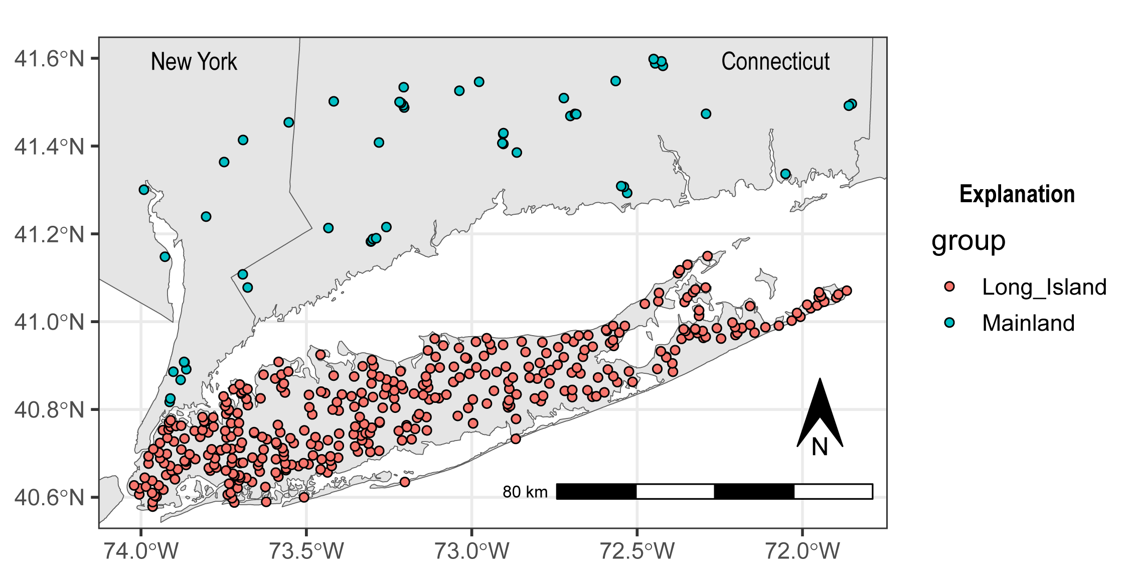
Create a timestep grid:
ARCHI organizes input data into a grid where the rows are timesteps and the columns are site identifiers. Timestep frequency can be annual, seasonal, monthly, weekly, or daily. Observed values falling into discretized timesteps are aggregated by median, mean, min, max, or user-specified quantile. Sites with no observation values during a given timestep are populated with NAs. Data can also be aggregated by water years. All timestep outputs are indexed by calendar-year date.
# Gridding groundwater levels by monthly medians from 1975 to 2022
grid <- timestep_grid(data =  LI_data,
                      timestep = "monthly",
                      agg_method = "median",
                      year_range = c(1975, 2022))

# The timestep index column contains dates representing the first day of the timestep by default
grid$timestep[1:5]
#> [1] "1975-01-01" "1975-02-01" "1975-03-01" "1975-04-01" "1975-05-01"
# We can use ARCHI to visualize dataset-scale missingness patterns
# and relative fluctuations in observation values over time
input_heatmap <- grid_heatmap(grid =  grid,
# Only include sites in the plot that are at least 35% complete
                             data_thresh = 0.35,
# Saturate colorbar scale within 3 standard deviations of mean
                             cb_rng = c(-3,3),
# Plot sites in order of completeness
                             order = "completeness")

plot(input_heatmap$grid_plot)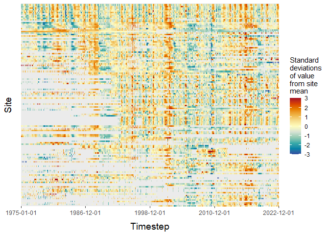
Trim timestep grid:
We can use ARCHI to trim the timestep grid before imputation. This removes sites with low proportions of observed values compared to the total number of gridded timesteps, which could result in potentially spurious regression models. Additionally, any timesteps that have no observed values across all sites are removed.
# Trim grid to remove sites with less than 35 percent observed values
grid <- trim_grid(input_grid = grid,
                  data_thresh = 0.35)
#> 339 site(s) removed with proportion complete less than site-data threshold of 0.35
Impute timestep grid:
ARCHI employs imputations using three different regression models: ordinary least squares (OLS), ridge regression (ridge), and maintenance of variance extension, type 1 (MOVE.1). An error method and threshold must be specified in order to accept model values for imputation. Here, we use the Nash-Sutcliffe efficiency (NSE) with an error threshold of 0, indicating regression models will not be accepted for imputation if they perform worse than mean imputation. More details on regression models and error thresholds included in ARCHI can be found in package documentation (?impute_grid()).
The maximum number of reference sites,n_refwl, must also be set. Here, we specify that the top 10 most correlated reference sites are used to impute the target. The default setting for n_refwl is "max", which uses all available correlated sites as references. If the default setting is used, the maximum number of reference sites can be further constrained as a proportion of the number of training observations using the p_per_n parameter. As a first order approximation, p_per_n values of 0.1 and 0.5 are recommended for OLS and ridge models, respectively, to avoid over-fitting and over-regularization. The MOVE.1 model only allows one reference site per regression model.
# Impute grid using ridge regression on top 10 most correlated reference sites
mod_out <- impute_grid(input_grid = grid,
                       model = "ridge",
                       error_method = "NSE",
                       error_thresh = 0,
                       n_refwl = 10)
#> Begin initial imputation: 39.46 percent NAs remaining...
#> Iteration 1 complete: 0 percent NAs remaining
#> Iteration 2 complete: 0 percent NAs remaining
#> Begin final pass: overwriting initial imputations with improved models...
#> Iteration 3 complete: 0 percent NAs remaining
#> Records attempted for imputation =  137
#> Incomplete records remaining =  0
#> Time difference of 12.76325 secs
Explore results:
# View the imputed grid using site order from original grid for direct comparison
imputed_heatmap <- grid_heatmap(grid = mod_out$imputed_grid,
                                order = "custom",
                                site_order = input_heatmap$site_order,
                                cb_rng = c(-3,3))

plot(imputed_heatmap$grid_plot)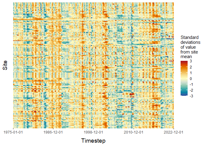
# We can view imputation results for a specified target site
# The top two correlated reference sites are included in below panels
ts_plots(impute_output = mod_out,
         site_no = "405827072190501",
         yax_lab = "Groundwater level, in feet below land surface",
         show_topn = c(1:2))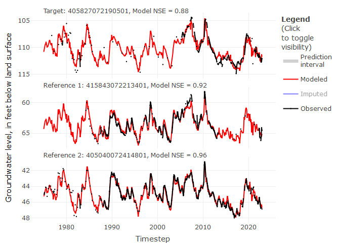
# We can also assess the residuals for this site
resid_plots(impute_output = mod_out,
         site_no = "405827072190501",
         plot_type = "marginal")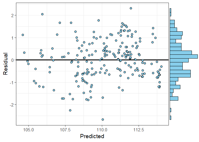
# We can organize the site order of the heatmap to group sites with similar time-series patterns
clustered_heatmap <- grid_heatmap(grid = mod_out$imputed_grid,
                                order = "cluster",
                                cb_rng = c(-3,3))

plot(clustered_heatmap$grid_plot)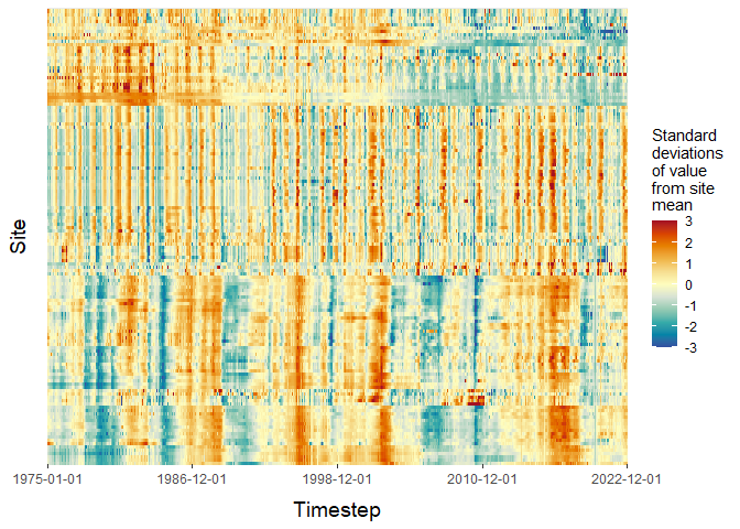
# We can also perform time-series clustering on complete records in a timestep grid
clust <- cluster_grid(input_grid = mod_out$imputed_grid)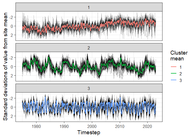
Evaluate model:
ARCHI can partition random observations in the timestep grid as “holdout data” with which to evaluate model results.
# Create random holdout grid by coercing 5 percent of observed values in input grid to NAs
hold <- hold_grid(grid, p = 0.05)

# Run model using the holdout grid
hold_mod_out <- impute_grid(input_grid = hold,
                            model = "ridge",
                            error_method = "NSE",
                            error_thresh = 0,
                            n_refwl = 10)
# Evaluate imputed holdouts vs "true" observed data
eval <- hold_eval(true = grid,
                  imp = hold_mod_out$imputed_grid,
                  hold = hold)
#> 100 percent of holdout values successfully imputed
# Plot holdout evaluation results with 1:1 line and RMSE
plot(eval$comp$Observed, eval$comp$Imputed,
     xlab = "Observed depth to groundwater, in feet",
     ylab = "Imputed depth to groundwater, in feet",
     cex.lab = 1.4, cex.axis = 1.2, cex.main = 1.4,
     main = paste0("Holdout RMSE = ", round(eval$rmse, digits = 2),
                   " feet (n = ", length(na.omit(eval$diff)),")"))
abline(0, 1, lty= 2, lwd = 2, col = "red")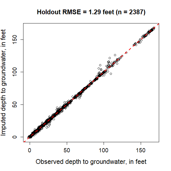
Export results:
An imputed model grid and performance statistics are included in the impute_grid() output. Also included is a long-format version of the imputed_grid output data frame that is easily exported from R and combined with other datasets. The out_long data frame includes timestep-aggregated observations and imputed values (attributed under the value_type field). Prediction intervals are included. Additionally, time_range indicates whether an imputed value is within (“Gap_fill”) or outside (“Extension”) the training period. The data_range field indicates whether an imputed value is within (“Interpolation”) or outside (“Extrapolation”) the range of the training data.
# View long format output
str(mod_out$out_long)
#> 'data.frame': 78912 obs. of 8 variables:
#> $ site_no : chr "403517073430702" "403517073430702" "403517073430702" "403517073430702" ...
#> $ timestep : Date, format: "1982-04-01" "1983-12-01" ...
#> $ value : num 16.1 15.5 14.4 15.3 15.1 ...
#> $ PI_lwr : num NA NA NA NA NA NA NA NA NA NA ...
#> $ PI_upr : num NA NA NA NA NA NA NA NA NA NA ...
#> $ data_range: chr "Interpolation" "Interpolation" "Interpolation" "Interpolation" ...
#> $ time_range: chr "Gap_fill" "Gap_fill" "Gap_fill" "Gap_fill" ...
#> $ value_type: chr "Imputed" "Imputed" "Imputed" "Imputed" ...
# Write output as csv file to working directory
write.csv(mod_out$out_long, "out_long.csv", row.names = F)
Additional functionality
Applying cutoffs:
Optional cutoffs can be applied to constrain reference sites used for imputation.
# Note: Distance cutoff and grouping methods require input of a `sites` data frame

# Only use references within 20 kilometers of a given target site
mod_20km <- impute_grid(input_grid = grid,
                        sites = LI_sites,
                        sites_crs = "NAD83",
                        d_cutoff = 20)

# Only use references within target's group
mod_grp <- impute_grid(input_grid = grid,
                        sites = LI_sites,
                        group_sites = T)

# Only use references with Pearson's correlation coefficients to target of 0.7 or higher
mod_corr <- impute_grid(input_grid = grid,
                        r_cutoff = 0.7)
Prediction intervals:
ARCHI includes a non-parametric bootstrapping routine for generation of prediction intervals for all included regression models. More information on the non-parametric bootstrap is provided by Mougan and Nielsen, 2022. It is recommended to set final_pass to FALSE for more robust prediction intervals, which may result in decreased imputation accuracy.
# Non-parametric bootstrap to calculate 95% prediction intervals (PIs) for ridge models
# with 500 random iterations (B) per site. Holdout dataset is used to evaluate PIs.
# Bootstrapping prediction intervals may take considerable computing time.
mod_boot <- impute_grid(input_grid = hold,
                        model = "ridge",
                        error_method = "NSE",
                        error_thresh = 0,
                        n_refwl = 10,
                        final_pass = F,
                        bootstrap_PI = T,
                        PI_alpha = 0.05,
                        B = 500,
                        verbose = F) # suppress messages to console
#> Time difference of 4.207747 mins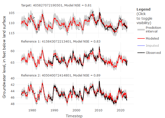
We can evaluate the coverage rate (CR) for bootstrapped prediction intervals generated from the holdout dataset, which is the proportion of the holdout observations within the prediction interval. The target CR for a 95% prediction interval is 0.95 or greater.
# Pass computed prediction intervals to hold_eval function
boot_eval <- hold_eval(true = grid,
                       imp = mod_boot$imputed_grid,
                       hold = hold,
                       PI_upr = mod_boot$PI_upr,
                       PI_lwr = mod_boot$PI_lwr)

# Print coverage rate
boot_eval$CR
#> [1] 0.9589443

# Print RMSE (now with final pass turned off)
boot_eval$rmse
#> [1] 1.39107
The computed coverage rate indicates about 95 percent of holdout datapoints were within respective prediction intervals. However, a slight increase of holdout RMSE indicates imputation accuracy decreased when the final_pass was deactivated. The final_pass generally tends to improve imputation accuracy, but can introduce data leakage which may lead to overoptimistic model fits and truncated prediction intervals. More information on the final_pass setting can be found in package documentation (?impute_grid()).
Installation of R and RStudio
To use the ARCHI package, you will need to have R and RStudio installed on your computer. This installation will only need to be done once for each computer. This link has instructions for installing R and RStudio:
R and RStudio Installation Instructions
Useful links:
USGS Software Release Information
https://doi.org/10.5066/P1VVHWKE
USGS Information Product Data System (IPDS): IP-163390
References
Evans, S.W., Jones, N.L., Williams, G.P., Ames, D.P., and Nelson, E.J., 2020, Groundwater Level Mapping Tool: An open source web application for assessing groundwater sustainability: Environmental Modelling and Software, 131, 104782, https://doi.org/10.1016/j.envsoft.2020.104782.
Hastie, T., 2020, Ridge Regularization: An Essential Concept in Data Science: Technometrics, v. 62, no. 4, p. 426-433, https://doi.org/10.1080/00401706.2020.1791959.
Hirsch, R.M., 1982, A comparison of four streamflow record extension techniques: Water Resources Research, v. 18, p. 1081–1088, https://doi.org/10.1029/WR018i004p01081.
Mougan, C., and Nielsen, D.S., 2022, Monitoring Model Deterioration with Explainable Uncertainty Estimation via Non-parametric Bootstrap. Proceedings of the AAAI Conference on Artificial Intelligence 1686, 15037-15045, https://doi.org/10.1609/aaai.v37i12.26755.
Nash, J.E., and Sutcliffe, J.V., 1970, River flow forecasting through conceptual models part I — A discussion of principles: Journal of Hydrology, v. 10, no. 3, p. 282–290, https://doi.org/10.1016/0022-1694(70)90255-6.
Rousseeuw, P.J., 1987. Silhouettes: A graphical aid to the interpretation and validation of cluster analysis: Journal of Computational and Applied Mathematics v. 20, 53–65, https://doi.org/10.1016/0377-0427(87)90125-7.
van Buuren, S., 2018, Flexible Imputation of Missing Data, Second Edition, CRC Press, Boca Raton. https://doi.org/10.1201/9780429492259.
U.S. Geological Survey, 2024, National Water Information System data available on the World Wide Web (USGS Water Data for the Nation), accessed February 12, 2024, at http://dx.doi.org/10.5066/F7P55KJN.
Disclaimer
This software is preliminary or provisional and is subject to revision. It is being provided to meet the need for timely best science. The software has not received final approval by the U.S. Geological Survey (USGS). No warranty, expressed or implied, is made by the USGS or the U.S. Government as to the functionality of the software and related material nor shall the fact of release constitute any such warranty. The software is provided on the condition that neither the USGS nor the U.S. Government shall be held liable for any damages resulting from the authorized or unauthorized use of the software.
Any use of trade, firm, or product names is for descriptive purposes only and does not imply endorsement by the U.S. Government.